Meta-analysis methods and formulas

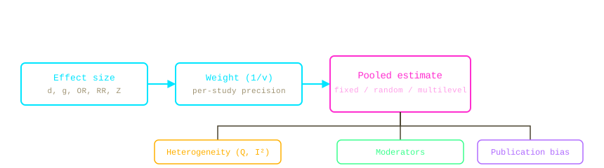
This page collects the most common formulas behind each step of a meta-analysis described in Meta-analysis steps — enough to understand how the numbers are actually computed, not an exhaustive reference. ProMeta implements a much wider range of formulas, covering many more effect-size types, models, and edge cases than shown here. In all formulas below, k is the number of studies, and each study i contributes an effect size (Y with subscript i) and its variance (v with subscript i).

Effect sizes based on means

Cohen's d standardizes the raw difference between two group means using the pooled standard deviation:

d = \frac{M_{1} - M_{2}}{{SD}_{pooled}}

{SD}_{pooled} = \sqrt{\frac{(n_{1} - 1) {SD}_{1}^{2} + (n_{2} - 1) {SD}_{2}^{2}}{n_{1} + n_{2} - 2}}

Cohen's d is slightly biased in small samples. Hedges' g corrects for this with a small-sample correction factor J:

g = d \times J, J = 1 - \frac{3}{4 df - 1}

The variance of d (needed to weight the study in the pooled analysis) is:

v_{d} = \frac{n_{1} + n_{2}}{n_{1} n_{2}} + \frac{d^{2}}{2 (n_{1} + n_{2})}

Effect sizes based on binary data

For a 2×2 table of a study (a, b, c, d = cell counts), the log odds ratio and its variance are:

\ln (OR) = \ln \frac{a d}{b c}

v_{\ln (OR)} = \frac{1}{a} + \frac{1}{b} + \frac{1}{c} + \frac{1}{d}

The log risk ratio, computed on the same table, is:

\ln (RR) = \ln \frac{\frac{a}{a + b}}{\frac{c}{c + d}}

Both are analyzed on the log scale (where sampling distributions are closer to normal) and only exponentiated back to OR/RR for reporting.

Effect sizes based on correlations

Pearson's r is not analyzed directly, since its sampling distribution is skewed for values far from zero. It is first converted to Fisher's Z:

Z_{r} = 0.5 \times \ln \frac{1 + r}{1 - r}

v_{Z_{r}} = \frac{1}{n - 3}

Pooled results are converted back to the r scale only at the end, for reporting.

Once an effect size is computed for every study, they still need to be combined into a pooled estimate — see Statistical models for the fixed-effect, random-effects, and multilevel models that do this, and the weights (w with subscript i) and pooled estimate (M) referenced below.

Heterogeneity

Q tests whether the observed variation across study effect sizes is larger than expected from sampling error alone (its null distribution is chi-squared with k − 1 degrees of freedom):

Q = \sum_{i = 1}^{k} w_{i} {(Y_{i} - M)}^{2}

Q is sensitive to the number of studies, so I² is used to quantify heterogeneity as a percentage of total variation, independent of k:

I^{2} = \max (0, \frac{Q - df}{Q}) \times 100 %

As a rule of thumb (Higgins & Thompson, 2002), I² around 25%, 50%, and 75% are considered low, moderate, and high heterogeneity — though this should always be read alongside the confidence interval around I², not as a hard cutoff.

Moderators

When a categorical moderator splits studies into p subgroups, Q decomposes into a between-subgroups component (does the moderator explain some of the heterogeneity?) and a within-subgroups component (how much heterogeneity remains inside each subgroup):

Q_{B} = \sum_{g = 1}^{p} w_{g} {(M_{g} - M)}^{2}

A continuous moderator is tested instead with a weighted meta-regression, where the effect size is regressed on the moderator using the same inverse-variance weights as the pooled model above.

Publication bias

Rosenthal's Fail-safe N estimates how many additional, unpublished null-result studies (averaging Z = 0) would need to exist to bring a significant pooled result down to non-significance:

N_{fs} = \frac{{(\sum_{i = 1}^{k} Z_{i})}^{2}}{2.706} - k

Fail-safe N only addresses one specific failure mode (studies missing entirely) and says nothing about selective outcome or analysis reporting within studies that were published. It is normally reported alongside, not instead of, a funnel plot and Egger's regression test (which regresses each study's standardized effect on its precision, testing whether smaller, less precise studies systematically report larger effects — the visual asymmetry a funnel plot shows).

Extensions

The methods above cover a single pairwise comparison per meta-analysis. Two situations call for an extended model:

More than two treatments/conditions being compared across the literature: see Network meta-analysis.
Single-subject data instead of group data: standard effect sizes don't apply — see Meta-analysis of single-case experimental designs.

References

The formulas above follow the notation and derivations in Borenstein, Hedges, Higgins, & Rothstein (2009), Introduction to meta-analysis — see the full reference list for further reading on each method.